Weighted spatial sampling

Weighted spatial sampling is a data generation method that uses context information to determine where points should be placed. Unlike simple random sampling (e.g. sf::st_sample), which trats every location equally and often results in accidental data clustering or large data gaps, a weighted design assigns different selection probabilities to different areas based on known characteristics, such as population density, elevation, or pollution.

Earlier geoimputation work used spatial sampling to improve geocoding accuracy. Unlike polygon centroids, weighted samples are located where people actually live and have locational variance, that is, the distance between each location is non-zero.

In this vignette, I show how weighted sampling works using counties in Colorado, USA, as an example.

library(geoimp)
library(tigris)
library(tidycensus)
library(sf)
library(dplyr)
set.seed(123)

co <- counties("CO", cb = TRUE, progress_bar = FALSE)
co_tracts <- tracts("CO", cb = TRUE, progress_bar = FALSE)
plot(co$geometry)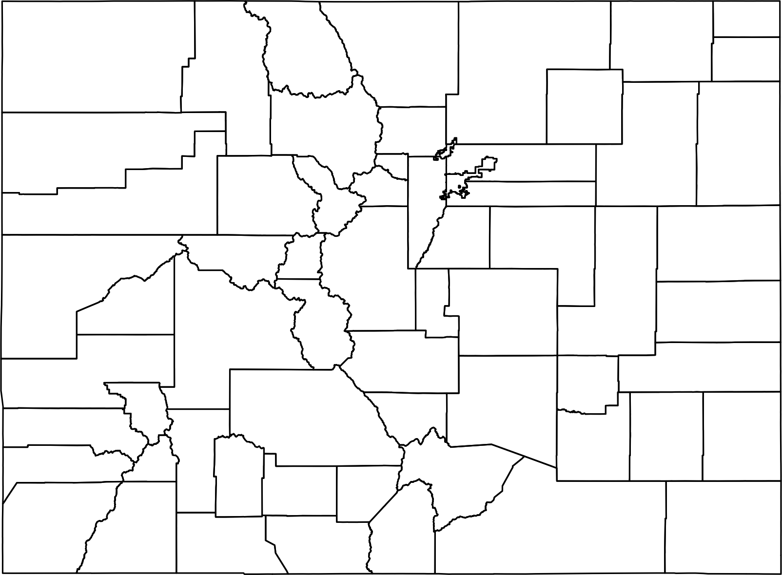

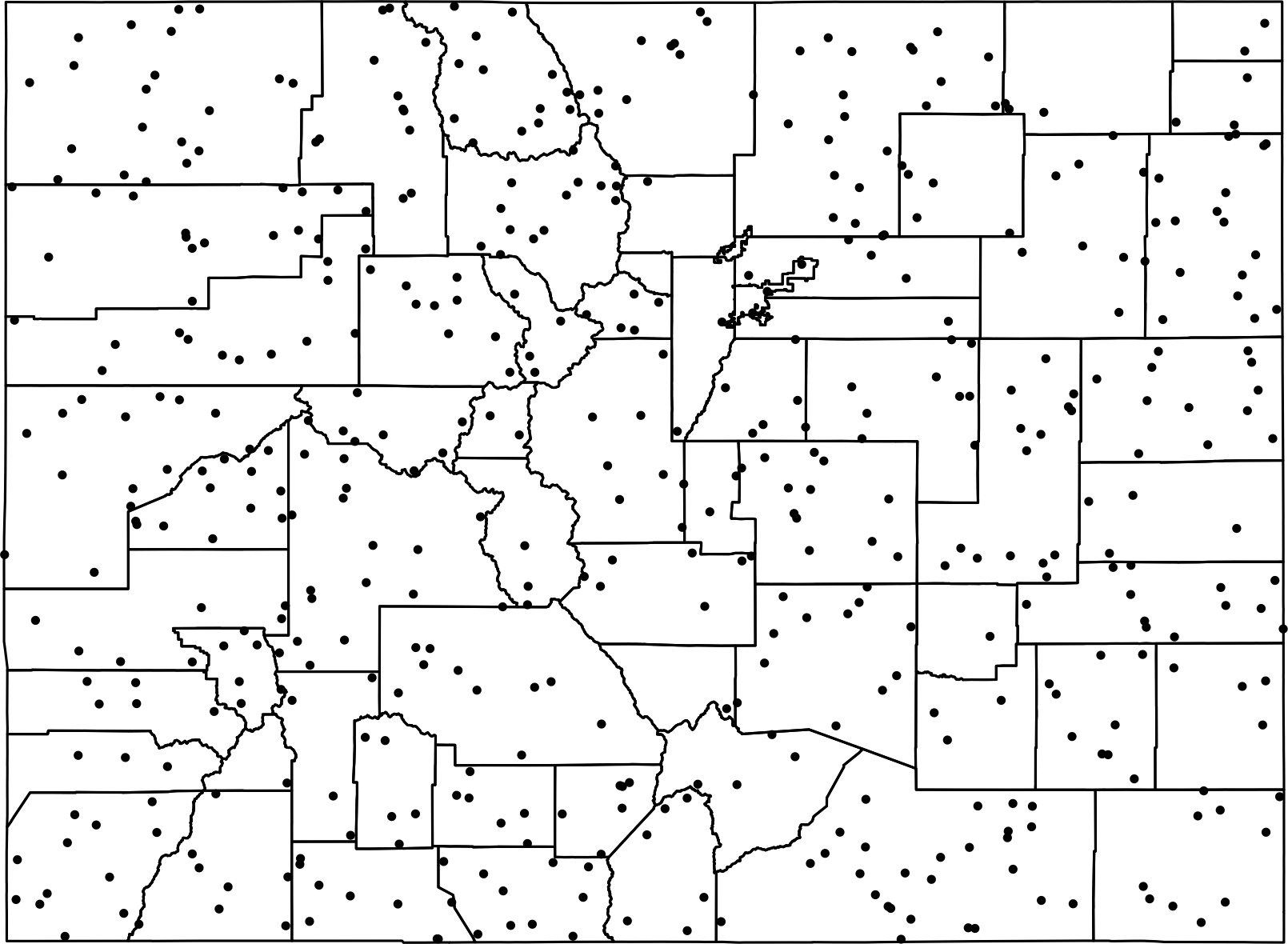
Simple spatial sampling produces a relatively even distribution of points, assigning a similar number of points to rural parts of outer Colorado and the Denver area in central Colorado.

smp <- st_sample(co, 500)
plot(co$geometry)
plot(smp, pch = 16, cex = 0.5, add = TRUE)

One popular way to sample with population weights is to sample by county polygon. Since region sizes often depend on the region’s population, this can lead to solid estimates. Of course, if region size and population are only spuriously or not at all correlated, the result is of low quality. To exemplify, take a look at Colorado’s counties (relatively evenly sized) and census tracts (roughly population-weighted).

smp <- st_sample(co, 500, by_polygon = TRUE)
plot(co$geometry)
plot(smp, pch = 16, cex = 0.5, add = TRUE)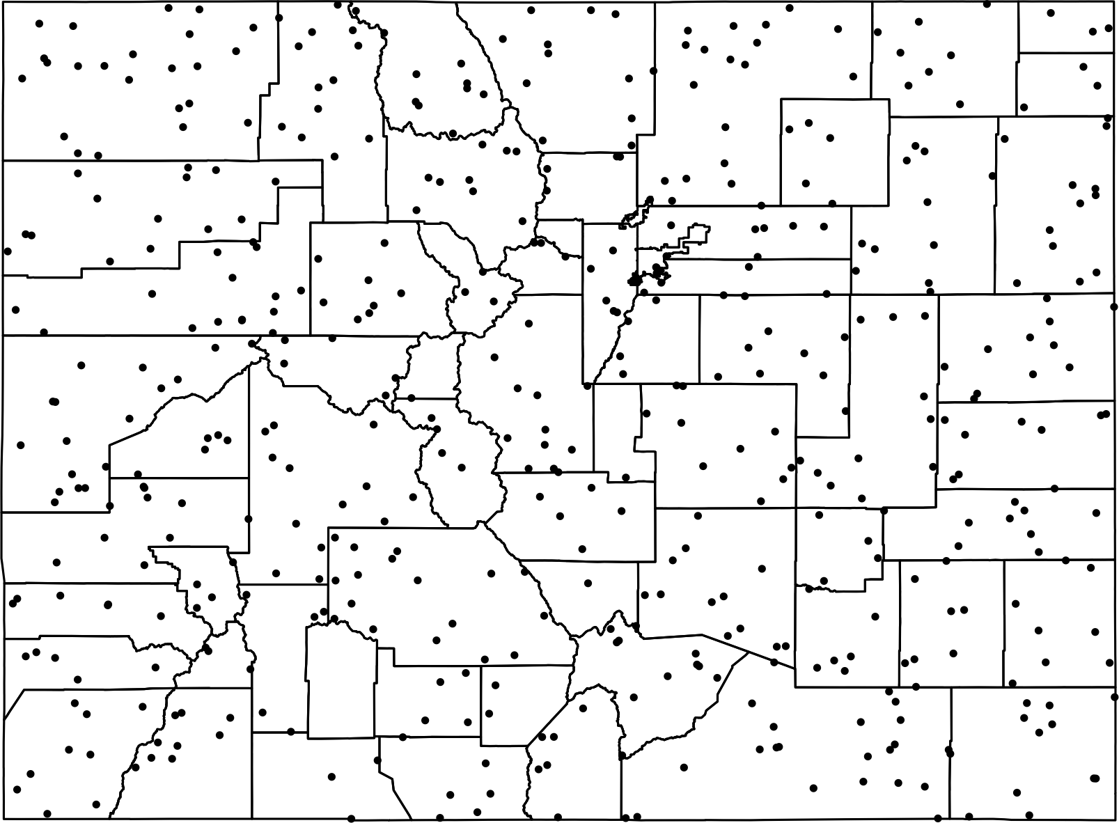

smp <- st_sample(co_tracts, 500, by_polygon = TRUE)
plot(co_tracts$geometry)
plot(smp, pch = 16, cex = 0.5, add = TRUE)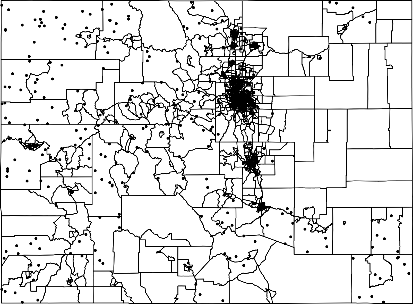

Since the Denver region has many times more census tracts than Colorado’s countryside, the probability of being sampled there is much higher.

For datasets with a less structured regional division, the wt_strata() function can create samples that are weighted by a covariate. To do this, we use population estimates from the Census Bureau.

co_pop <- get_estimates(
    geography = "county",
    product = "population",
    year = 2025,
    vintage = 2025,
    state = "CO",
    output = "wide",
    geometry = TRUE
)[c("GEOID", "POPESTIMATE")]

smp <- wt_sample(co_pop["POPESTIMATE"], size = 500)
plot(co_pop$geometry)
plot(smp, pch = 16, cex = 0.5, add = TRUE)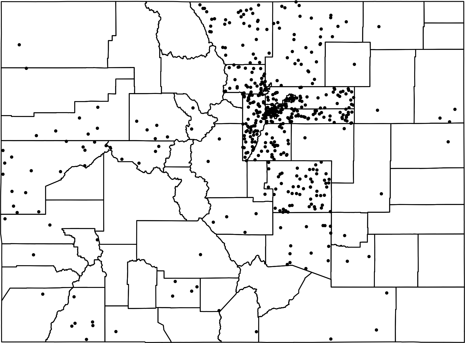

You can also control the degree of weighting. Decreasing the power argument decreases the “gravity” of high-value weights while increasing it, increases the gravity.

smp <- wt_sample(co_pop["POPESTIMATE"], size = 500, power = 0.5)
plot(co_pop$geometry)
plot(smp, pch = 16, cex = 0.5, add = TRUE)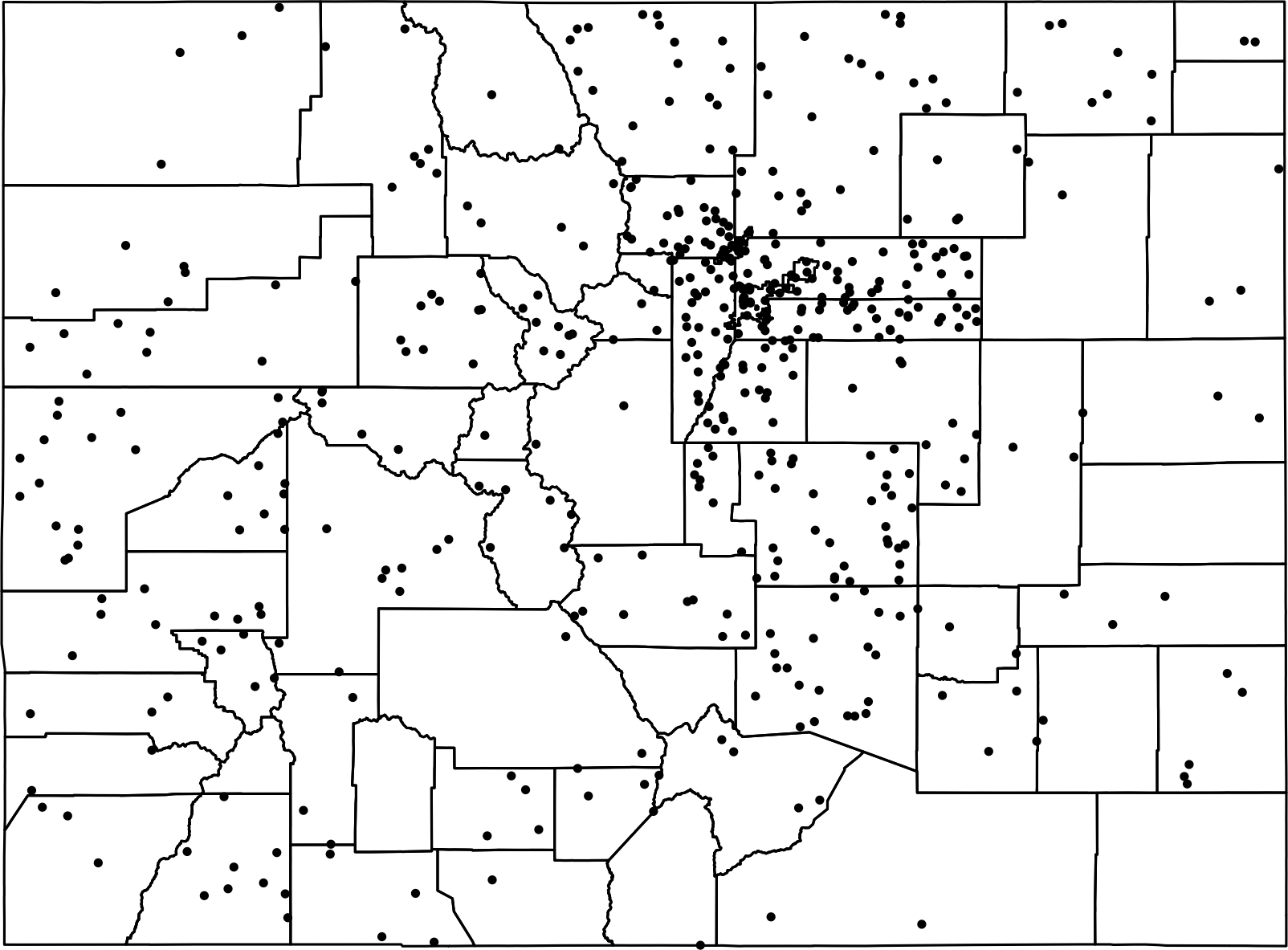

smp <- wt_sample(co_pop["POPESTIMATE"], size = 500, power = 2)
plot(co_pop$geometry)
plot(smp, pch = 16, cex = 0.5, add = TRUE)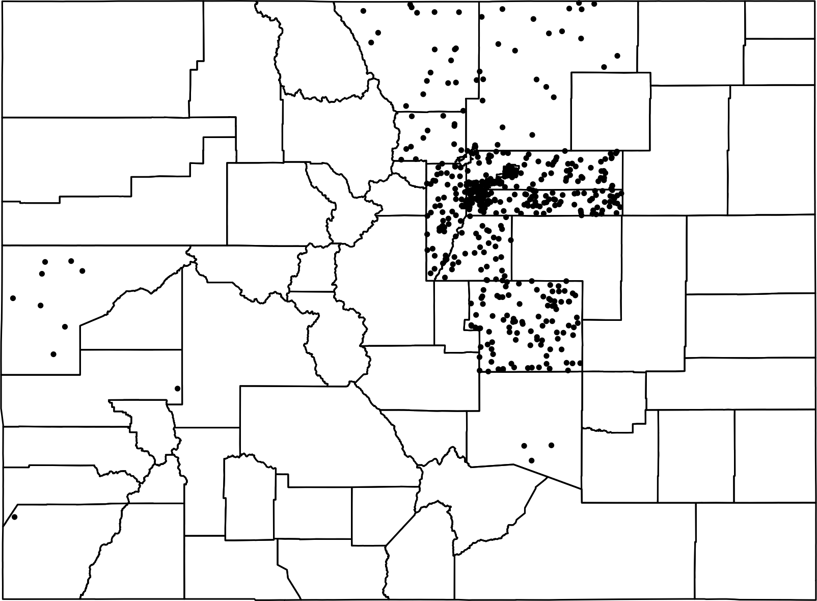

You can also use raster datasets as weights in wt_sample(). Combined with data providers like WorldPop or GHSL, this allows for a much more fine-grained weighting.

library(terra)
popgrid <- wp_data("USA")
popgrid <- crop(popgrid, co)

smp <- wt_sample(popgrid, 500)
plot(popgrid)
plot(smp, pch = 16, cex = 0.5, col = "white", add = TRUE)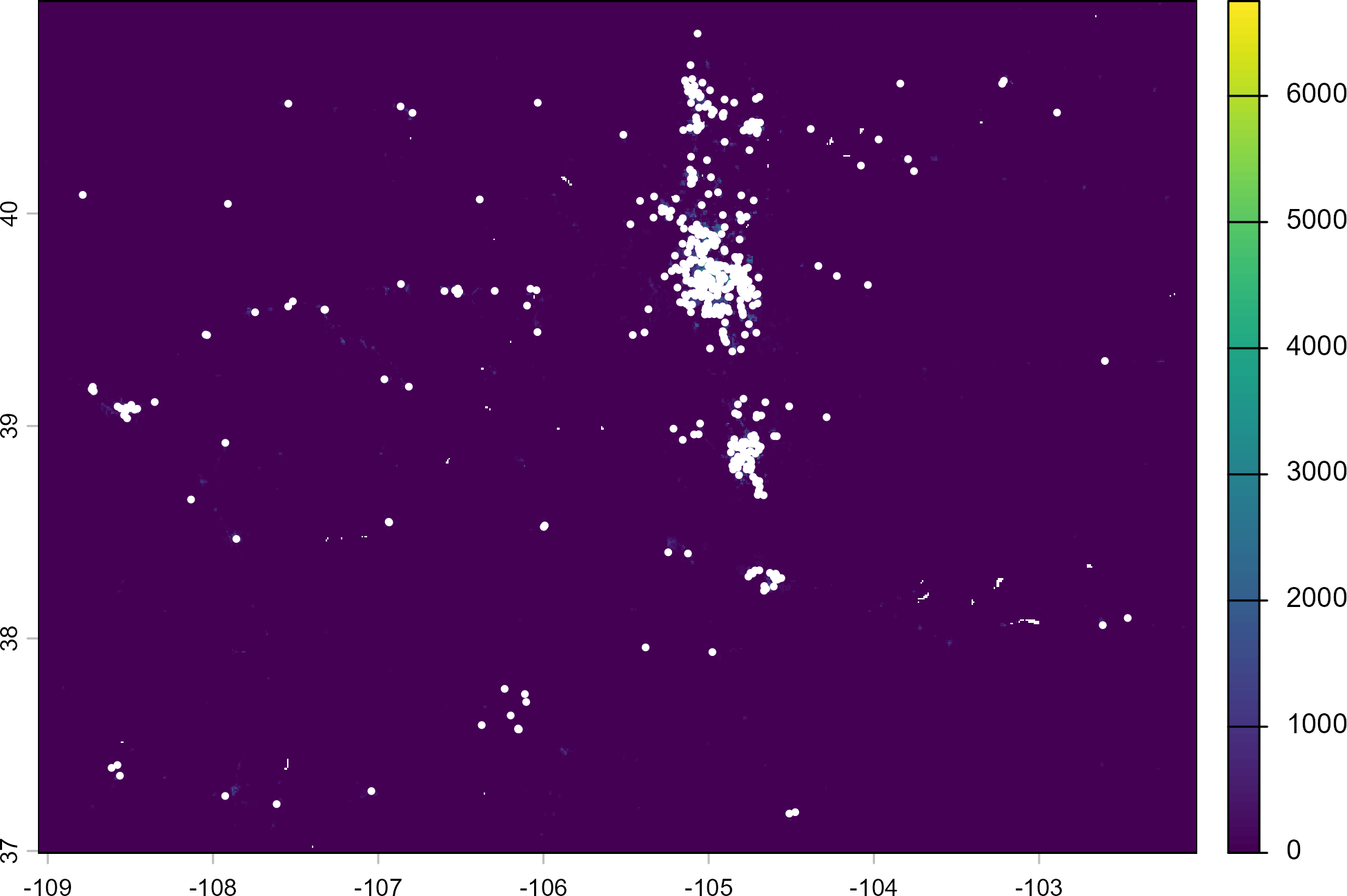

Finally, wt_sample provides tools to “de-bias” irregular geometries. If we wanted an unbiased (weighted) sample over all census tracts, we can add an area weight. In the following we compute a non-weighted sample (power = 0) and instead weight solely by the tract area. As you can see, the sample is relatively evenly distributed despite the clear geometrical bias of the census tracts.

smp <- wt_sample(co_tracts["ALAND"], power = 0, size = 500, area_weight = 1)
plot(co_tracts$geometry)
plot(smp, pch = 16, cex = 0.5, add = TRUE)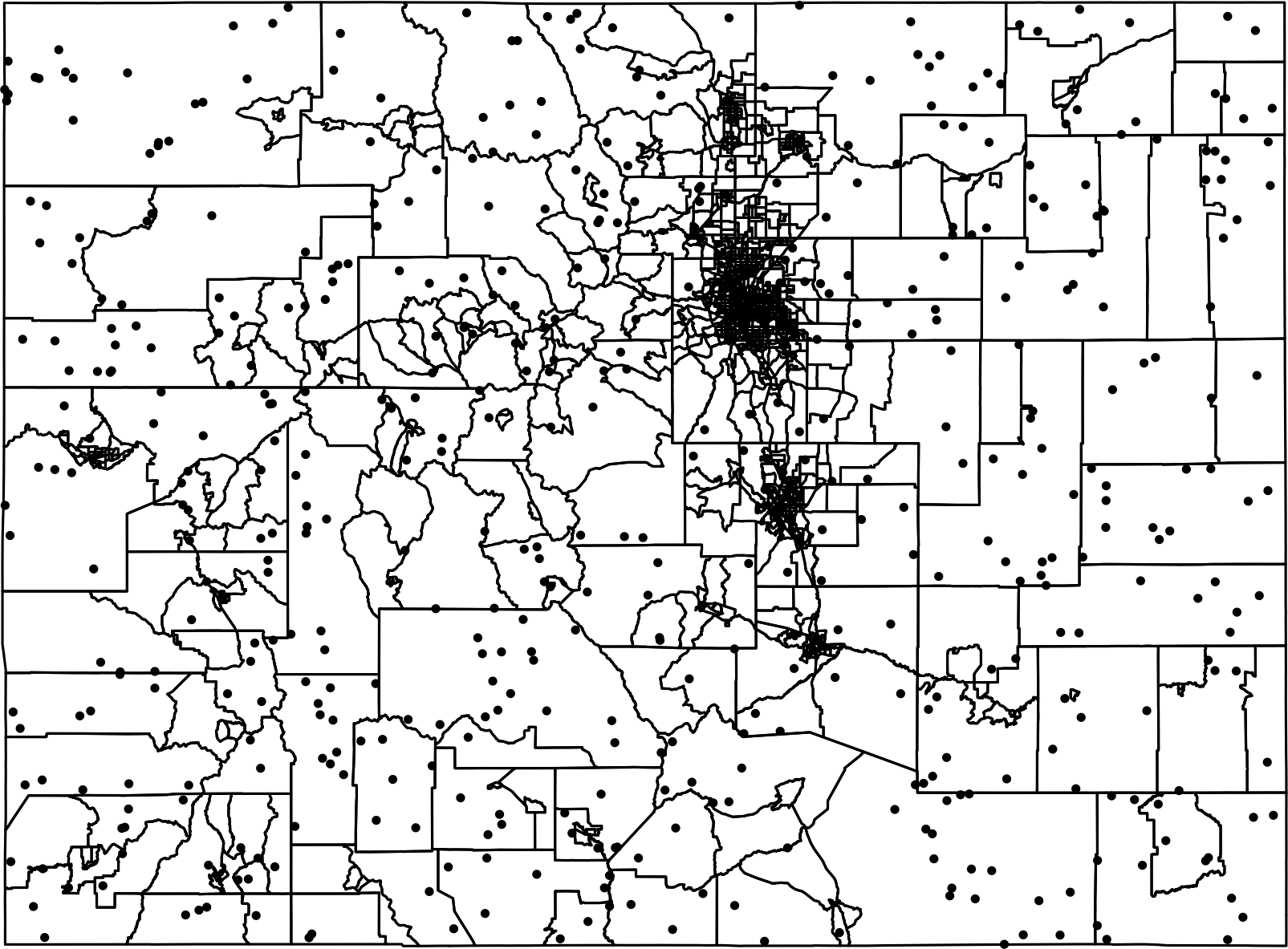

Weighted sampling is a powerful method and has been applied numerous times in spatial statistics. However, it’s still mostly random and unrelated to the subject of study. For example, when we know about the type of residence or the income of a geocoded subject, we can further refine the geocoded location. See the vignette “Introduction to geoimputation” for ways to link context data and personal data.