
Survey respondents are commonly linked to geographic areas rather than precise addresses, both to protect privacy and because precise locations are often unavailable. A respondent might be assigned to their municipality, electoral district, or county represented as a single point at the area’s centroid. While this is sufficient for many analyses, it becomes a problem whenever location actually matters: spatial modeling, neighbourhood context, or any analysis that requires knowing where within an area someone lives.
Geoimputation addresses this by probabilistically assigning each respondent a plausible location within their area, using auxiliary spatial data (e.g., population density, land cover, built-up area)d as a guide. The result is not a known location, but a statistically principled one that respects both the area boundaries and whatever contextual information respondents provided about their surroundings (e.g., “I live in a village” or “I live in a large city”).
Imagine you have georeferenced survey data containing items on income and rurality.
library(geoimp)
library(sf)
library(terra)

dummy <- dummy_data()
dummy$survey
#> Simple feature collection with 50 features and 2 fields
#> Geometry type: POINT
#> Dimension:     XY
#> Bounding box:  xmin: 1.166667 ymin: 1.166667 xmax: 2.833333 ymax: 2.833333
#> Projected CRS: +proj=tmerc +lat_0=0 +lon_0=0 +k=1 +x_0=0 +y_0=0 +ellps=WGS84 +units=m +no_defs
#> First 10 features:
#>    place_type    income                  geometry
#> 1     Village 3001-4000 POINT (2.833333 1.166667)
#> 2     Village 3001-4000 POINT (2.833333 1.166667)
#> 3     Village 1001-2000 POINT (2.833333 1.166667)
#> 4        City    <=1000 POINT (2.833333 1.166667)
#> 5     Village 2001-3000 POINT (2.833333 1.166667)
#> 6     Village    <=1000 POINT (2.833333 1.166667)
#> 7        City    <=1000 POINT (2.833333 1.166667)
#> 8        Town 3001-4000 POINT (2.833333 1.166667)
#> 9     Village     >4000 POINT (2.833333 1.166667)
#> 10       City    <=1000 POINT (2.833333 1.166667)
As you can see, the coordinates are all the same, x: 2 / y: 2. The reason for this is that in the original survey dataset, each respondent was only assigned an administrative area identifier. Each respondent was georeferenced by linking these administrative area by their identifiers. This is a common step in survey research that ensures anonymity of survey respondents. The downside is that it results in something like this:
library(ggplot2)

ggplot() +
  geom_sf(data = dummy$areas, fill = NA) +
  geom_sf(data = dummy$survey, aes(color = income), size = 2) +
  scale_color_discrete("Income") +
  theme_void()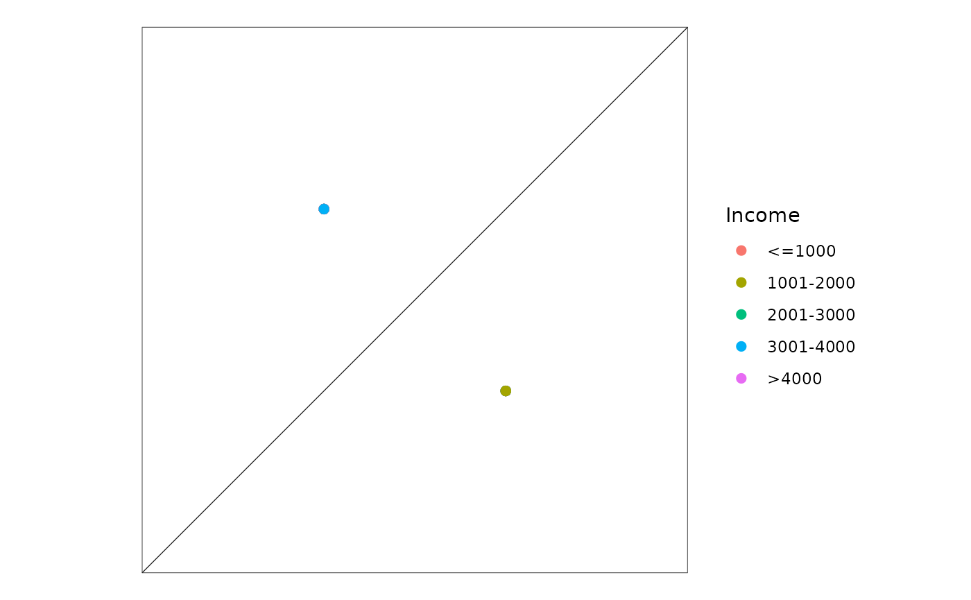
Each coordinate is the centroid (the center point) of their assigned administrative area. This means you cannot make out any spatial patterns, you cannot map the results and, most importantly, you cannot perform any spatial analysis or spatial modeling. Also, looking at where people actually live, we see:
library(tidyterra)
#>
#> Attaching package: 'tidyterra'
#> The following object is masked from 'package:stats':
#>
#>     filter

ggplot() +
  geom_spatraster(data = dummy$pop, aes(fill = pop)) +
  geom_sf(data = dummy$survey, aes(color = income), size = 2) +
  scale_fill_viridis_c("Population") +
  scale_color_discrete("Income") +
  guides(fill = guide_legend(order = 1), color = guide_legend(order = 2)) +
  theme_void()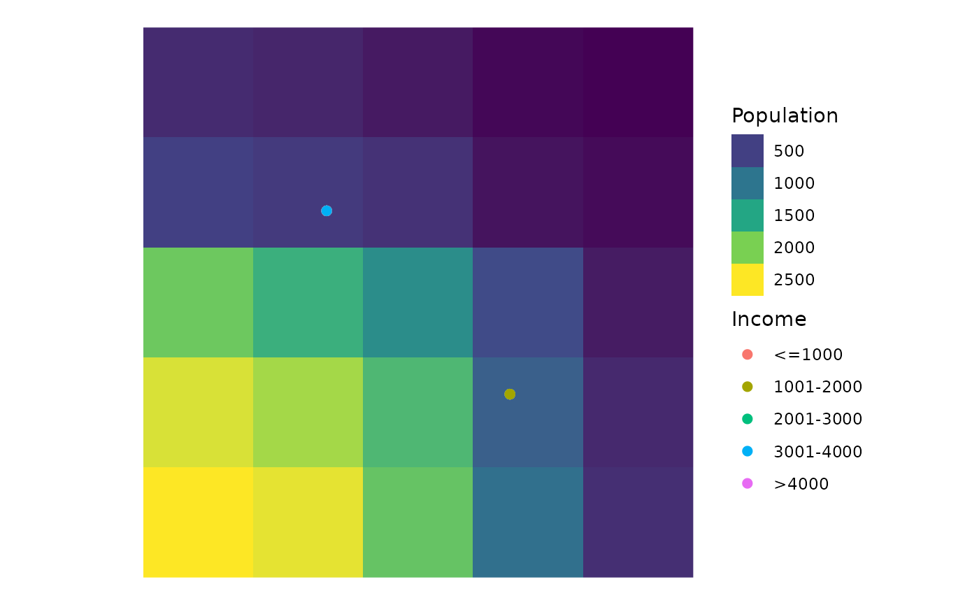
Neither of the centroids represent where the people in the survey live nor where people generally live. A traditional way to handle this is to compute a population-weighted centroid.
pop_centroid <- wt_centroid(dummy$areas, dummy$pop)

ggplot() +
  geom_spatraster(data = dummy$pop, aes(fill = pop)) +
  geom_sf(data = pop_centroid, size = 2) +
  scale_fill_viridis_c("Population") +
  theme_void()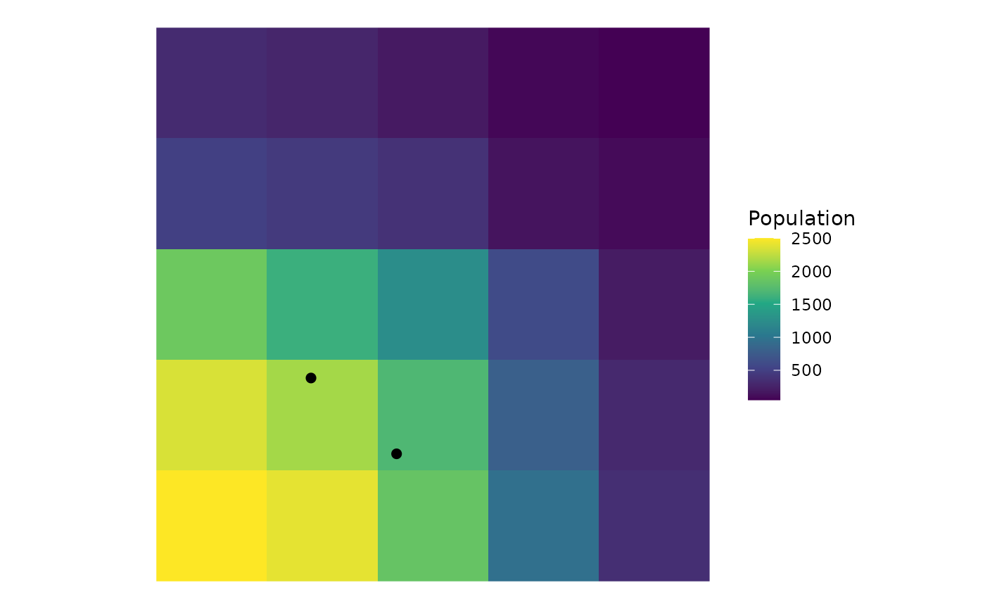
This solves one problem: centroids having no relation to their underlying context. But the points are still stacked on top of each other. Another way could be to do spatial sampling using population weights.
set.seed(123)
pop_sample <- wt_strata(dummy$survey, dummy$pop, psu = dummy$areas, method = "random")

ggplot() +
  geom_spatraster(data = dummy$pop, aes(fill = pop)) +
  geom_sf(data = pop_sample, aes(color = place_type), size = 2) +
  scale_fill_viridis_c("Population") +
  scale_color_discrete("Place type") +
  theme_void()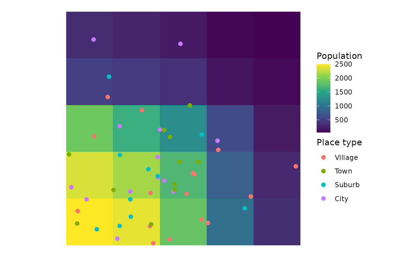
Now each respondent is spread out and the randomness is sort of controlled by specifying population weights. This allows us to do spatial analysis. But is it really meaningful? After all, we can see that some respondents who said they live in a village are sampled near the city center. Clearly, knowing where people generally live is not always enough.
The wt_strata() function allows you to link external
weights data with information from survey respondents. The goal is to
sample people who say they live in low-density areas only in low-density
areas. Or people who say they live in low-income areas only in
low-income areas. Or other combinations. To do this, you need a
“sampling schema” that links contextual information to surveyed
information. In other words, which population density corresponds to
which value in the survey item?
schema <- ssu_schema(
  Village = c(0, 200),
  Town = c(200, 600),
  Suburb = c(600, 1500),
  City = c(1500, Inf)
)
schema
#> SSU schema using fixed thresholds
#> Points are only sampled within these thresholds.
#>
#> Village = [0, 200)
#> Town    = [200, 600)
#> Suburb  = [600, 1500)
#> City    = [1500, Inf]
If you don’t know how exactly to construct a schema, you can use
proto_schema() to prototype schemas based on your data. For
final models, it probably makes sense to consult existing typologies or
base your schemas off empirical results, though.
When using the schema in wt_strata(), points are sampled
in grid cells of the population raster ranging between 0 and 200 people
if the survey respondent said they live in a village.
set.seed(123)
pop_geoimp <- wt_strata(
  dummy$survey,
  dummy$pop,
  psu = dummy$areas,
  ssu = dummy$survey$place_type,
  schema = schema,
  method = "random",
  replace = TRUE
)

ggplot() +
  geom_spatraster(data = dummy$pop, aes(fill = pop)) +
  geom_sf(data = pop_geoimp, aes(color = place_type), size = 2) +
  scale_fill_viridis_c("Population") +
  scale_color_discrete("Place type") +
  theme_void()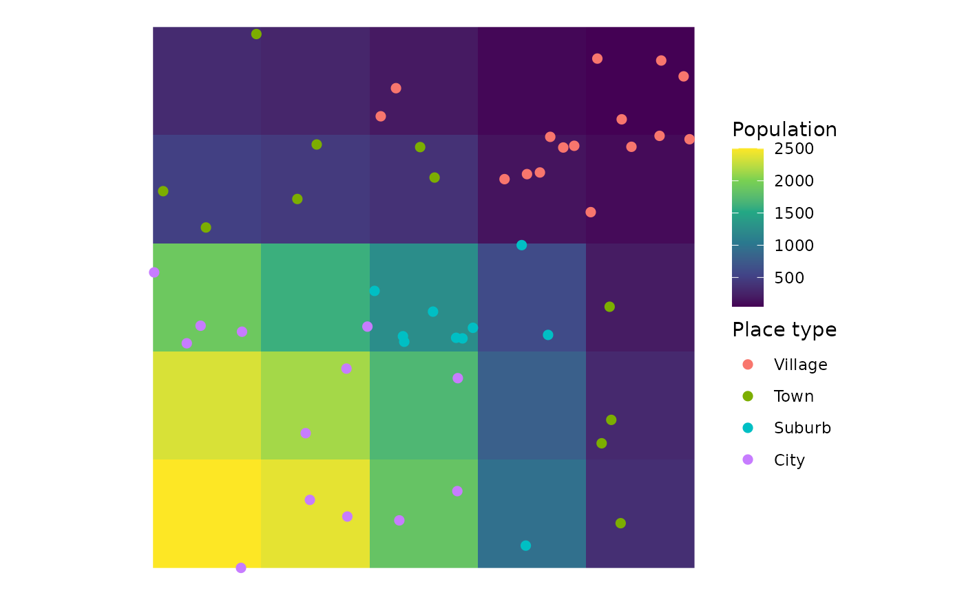
As you can see, the sampled points are not clustered around the population center anymore. Pink points (city dwellers) are clustered around the population center and orange points (rural dwellers) are clustered in the top-right corner where population density is low.
Of course, neither the raster nor the schema have to reference population data. The same could be done with any survey attribute that can be reasonably matched to any context data. For example, given a raster on income levels per cell:
ssu_schema(
  "<=1000" = c(0, 1000),
  "1001-2000" = c(1000, 2000),
  "2001-3000" = c(2000, 3000),
  "3001-4000" = c(3000, 4000),
  ">4000" = c(4000, Inf),
  closure = "right"
)
#> SSU schema using fixed thresholds
#> Points are only sampled within these thresholds.
#>
#> <=1000    = [0, 1000]
#> 1001-2000 = (1000, 2000]
#> 2001-3000 = (2000, 3000]
#> 3001-4000 = (3000, 4000]
#> >4000     = (4000, Inf]
The schema is not tied to population density or settlement type. Any survey item that can be matched to a spatial variable, whether that is income brackets, distance to the nearest urban center, or built-up area fraction. The closure = “right” argument adjusts which interval endpoint is inclusive, which matters when survey categories use <= or >= boundaries.