Geoimputation assigns respondents a location within their primary sampling unit based on auxiliary spatial data. Like any imputation, this process is stochastic: a different run produces different locations. Multiple geoimputation treats this uncertainty the same way multiple imputation treats missing data — by running the process \(m\) times, fitting the analysis model on each imputed dataset, and pooling the results using Rubin’s rules. The pooled estimates correctly reflect both the sampling variability of the analysis model and the uncertainty introduced by the unknown within-PSU location.
This vignette demonstrates the workflow using data from the German Longitudinal Election Study (GLES), a population density grid for Hesse, and federal electoral districts as primary sampling units.
library(geoimp)
library(terra)
library(tidyverse)
library(sf)

# Packages for multiple imputation
library(mice)
library(broom)
Retrieve population grid
popgrid
#> class       : SpatRaster
#> size        : 251, 175, 1  (nrow, ncol, nlyr)
#> resolution  : 1000, 1000  (x, y)
#> extent      : 4162000, 4337000, 2921000, 3172000  (xmin, xmax, ymin, ymax)
#> coord. ref. : ETRS89-extended / LAEA Europe (EPSG:3035)
#> source(s)   : memory
#> name        : cat_0
#> min value   :     3
#> max value   : 20067
Retrieve electoral districts
library(httr2)

req <- request("https://service.bundeswahlleiterin.de/") |>
  req_url_path("gis", "cgi-bin", "mapserv") |>
  req_url_query(
    map = "/home/fgs/gis/gisdocs/wahlkreise/wahlkreise2021wfs.map",
    service = "wfs",
    version = "1.0.0",
    request = "GetFeature",
    typename = "wahlkreise"
  )

elec_districts <- read_sf(req$url) |>
  filter(LAND_NAME == "Hessen") |>
  select(wkr = WKR_NAME, geometry = msGeometry) |>
  st_transform(3035) |>
  mutate(
    wkr = gsub("\u00df", "ss", wkr),
    wkr = gsub("\u2013", "-", wkr)
  )
elec_districts
#> Simple feature collection with 22 features and 1 field
#> Geometry type: MULTIPOLYGON
#> Dimension:     XY
#> Bounding box:  xmin: 4161511 ymin: 2920899 xmax: 4337501 ymax: 3172019
#> Projected CRS: ETRS89-extended / LAEA Europe
#> # A tibble: 22 × 2
#>    wkr                                                                         geometry
#>  * <chr>                                                             <MULTIPOLYGON [m]>
#>  1 Waldeck                              (((4287573 3168515, 4291271 3168332, 4291348 3…
#>  2 Kassel                               (((4287080 3143745, 4288034 3143352, 4288656 3…
#>  3 Werra-Meissner - Hersfeld-Rotenburg  (((4315810 3140144, 4315658 3139690, 4315677 3…
#>  4 Schwalm-Eder                         (((4280410 3124179, 4283102 3123876, 4284243 3…
#>  5 Marburg                              (((4248925 3092384, 4248829 3092212, 4248781 3…
#>  6 Lahn-Dill                            (((4205223 3083871, 4205521 3083780, 4205591 3…
#>  7 Giessen                              (((4261043 3080919, 4264741 3079283, 4265002 3…
#>  8 Fulda                                (((4315508 3071792, 4315824 3071664, 4316131 3…
#>  9 Main-Kinzig - Wetterau II - Schotten (((4269300 3045788, 4268431 3043152, 4268045 3…
#> 10 Hochtaunus                           (((4193565 3051782, 4193924 3051769, 4194427 3…
#> # ℹ 12 more rows
Retrieve GLES survey data
library(rgesis)
library(haven)

# Run authentication before downloading from GESIS data archive
# gesis_auth()

gles_cum <- gesis_get(paste0("ZA", 7709:7716)) |>
  lapply(function(record) {
    read_sav(gesis_data(
      record,
      download_purpose = "scientific_research",
      select = c("\\.sav", "main")
    )) |>
      select(starts_with("elecdist"), t1056, t40, t70)
  }) |>
  bind_rows()

gles_clean <- gles_cum |>
  select(
    starts_with("elecdist"),
    place_type = t1056,
    income = t70
  ) |>
  mutate(across(everything(), ~recode_values(
    .x,
    c(-99, -98, -94, -71, -72, -93) ~ NA,
    default = .x
  ))) |>
  mutate(across(everything(), as_factor)) |>
  mutate(
    place_type = fct_recode(
      place_type,
      "Large city" = "Grossstadt",
      "City/Suburb" = "Rand oder Vorort einer Grossstadt",
      "Town" = "Mittel- oder Kleinstadt",
      "Village" = "Laendliches Dorf",
      "Homestead" = "Einzelgehoeft oder alleinstehendes Haus auf dem Land"
    ),

    # translate income to english
    income = fct_relabel(
      income, ~gsub("bis", "to", .) |>
        gsub("unter", "<", x = _) |>
        gsub("Euro", "\u20ac", x = _)
      ) |>
      fct_recode(">= 10000 €" = "10000 € und mehr")
  ) %>%

  # merge different electoral district columns
  mutate(wkr = coalesce(!!!select(., starts_with("elecdist")))) %>%
  mutate(across(starts_with("elecdist"), ~NULL)) %>%
  drop_na() %>%

  # add geometries and drop all respondents outside of Hesse
  left_join(elec_districts, by = "wkr") |>
  filter(!st_is_empty(geometry))
#> Error in `UseMethod()`:
#> ! no applicable method for 'left_join' applied to an object of class "factor"

gles <- sf::st_centroid(st_as_sf(gles_clean), of_largest_polygon = TRUE)
gles
#> Simple feature collection with 665 features and 4 fields
#> Geometry type: POINT
#> Dimension:     XY
#> Bounding box:  xmin: 4185505 ymin: 2947487 xmax: 4309602 ymax: 3137857
#> Projected CRS: ETRS89-extended / LAEA Europe
#> # A tibble: 665 × 5
#>    place_type  pol_internet    income           wkr                    geometry
#>  * <fct>       <fct>           <fct>            <chr>               <POINT [m]>
#>  1 City/Suburb 3 days          2500 to < 3000 € Frankfurt am… (4220761 3002023)
#>  2 City/Suburb Less than 1 day 4000 to < 5000 € Kassel        (4288090 3132002)
#>  3 Large city  7 days          1000 to < 1250 € Frankfurt am… (4225547 3001206)
#>  4 Town        4 days          1000 to < 1250 € Marburg       (4232175 3081373)
#>  5 City/Suburb 5 days          2000 to < 2500 € Kassel        (4288090 3132002)
#>  6 Large city  7 days          1250 to < 1500 € Offenbach     (4231330 2992853)
#>  7 Large city  7 days          3000 to < 4000 € Frankfurt am… (4220761 3002023)
#>  8 Large city  2 days          1250 to < 1500 € Frankfurt am… (4220761 3002023)
#>  9 Village     3 days          2000 to < 2500 € Werra-Meissn… (4309602 3103814)
#> 10 Large city  3 days          1250 to < 1500 € Marburg       (4232175 3081373)
#> # ℹ 655 more rows
Together the data looks as follows. The georeferenced points are at the centroid of their municipality.
Code for dataset map
popgrid_df <- as.data.frame(popgrid, xy = TRUE)

ggplot() +
  geom_tile(data = popgrid_df, aes(x, y, fill = cat_0), color = NA) +
  geom_sf(data = elec_districts, fill = NA) +
  geom_sf(data = gles) +
  coord_sf(crs = 3035) +
  scale_color_continuous(labels = \(x) levels(gles$income)[round(x)]) +
  scale_fill_gradientn(
    colors = c(
      "#FFFFFF", "#FFBA5A", "#5A0400"
    ),
    transform = scales::transform_boxcox(0.5)
  ) +
  labs(x = NULL, y = NULL, fill = "Population") +
  theme_void()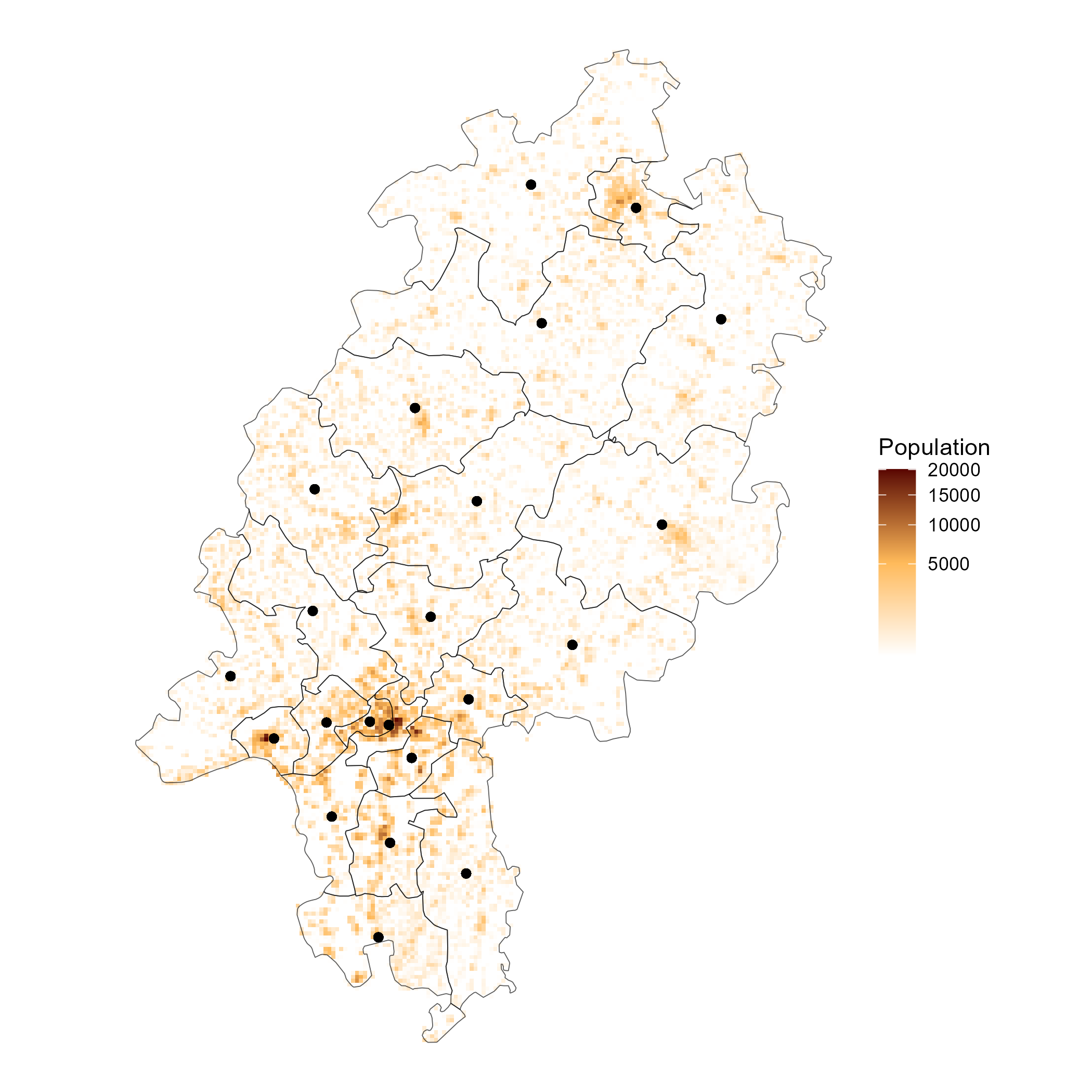
Multiple geoimputation
Each respondent reported their settlement type (homestead, village,
town, city/suburb, or large city). We define a fixed schema that maps
each settlement type to a population density range, so that
geoimputation places respondents in cells consistent with their
self-report. Running wt_strata() 50 times produces 50
datasets, each with a different draw of plausible locations.
schema_fixed <- ssu_schema(
  Homestead = c(0, 20),
  Village = c(20, 500),
  Town = c(500, 1000),
  `City/Suburb` = c(1000, 2000),
  `Large city` = c(2000, Inf)
)

set.seed(123)
imp_mi <- lapply(1:50, function(i) {
  wt_strata(
    gles,
    weights = popgrid,
    psu = elec_districts,
    ssu = gles$place_type,
    schema = schema_fixed,
    replace = TRUE,
    method = "random"
  )
})
The following map depicts the first of these geoimputed datasets. We computed 49 more of these datasets with different randomizations. None of these datasets represents the “truth”, but each of them are possible scenarios that multiple imputation can pool to a more robust solution.
Code for geoimputed map
ggplot() +
  geom_tile(data = popgrid_df, aes(x, y, fill = cat_0), color = NA) +
  geom_sf(data = elec_districts, fill = NA) +
  geom_sf(data = imp_mi[[1]], aes(color = as.numeric(income))) +
  coord_sf(crs = 3035) +
  scale_color_viridis_c(
    labels = \(x) levels(gles$income)[round(x)],
    option = "G"
) +
  scale_fill_gradientn(
    colors = c(
      "#FFFFFF", "#FFBA5A", "#5A0400"
    ),
    transform = scales::transform_boxcox(0.5)
  ) +
  labs(x = NULL, y = NULL, fill = "Population", color = "Income") +
  theme_void() +
  theme(legend.spacing.y = unit(0.8, "cm"))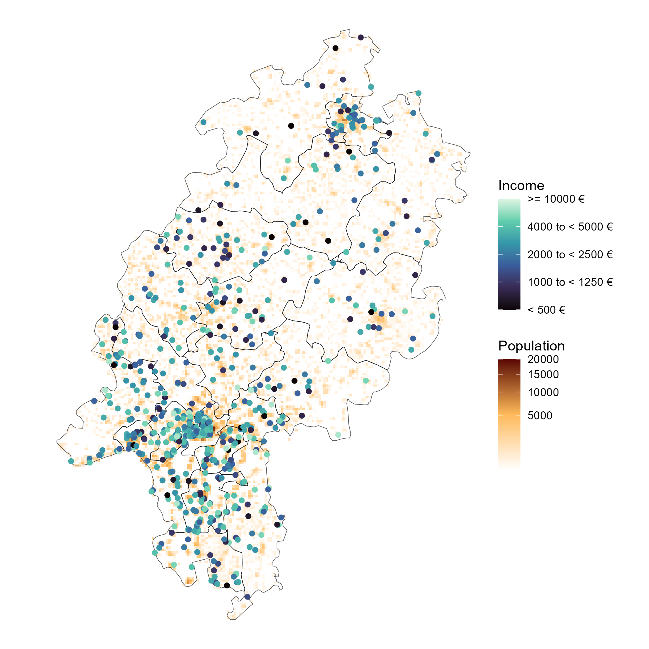
Analysis: does local rent predict income?
As an illustration, we estimate the association between the average rent in a respondent’s neighbourhood and their individual income. The key question is how the spatial resolution of “neighbourhood” affects the estimate. We compare three approaches:
- Centroid: all respondents are placed at their electoral district centroid; rent is averaged to the district level. This is the standard approach when individual locations are unknown.
- Single geoimputation: respondents are placed at one imputed location; rent is taken from the nearest grid cell. Finer spatial resolution, but location uncertainty is ignored.
- Multiple geoimputation: 50 imputed locations per respondent; rent is extracted at each, and results are pooled with Rubin’s rules. Finer resolution and honest uncertainty propagation.
rent <- z22_data("rent_avg", as = "sf") |>
  rename(rent = cat_0)

rent_agg <- aggregate(rent, elec_districts, FUN = mean, join = st_contains) |>
  st_join(elec_districts, join = st_equals) |>
  st_drop_geometry()
modgles <- gles
modgles <- left_join(modgles, rent_agg, by = "wkr")
modgles$income <- as.numeric(modgles$income)
The centroid baseline uses district-averaged rent and ignores within-district spatial variation.
res_agg <- tidy(lm(income ~ rent, data = modgles), conf.int = TRUE)
res_agg
#> # A tibble: 2 × 7
#>   term        estimate std.error statistic  p.value conf.low conf.high
#>   <chr>          <dbl>     <dbl>     <dbl>    <dbl>    <dbl>     <dbl>
#> 1 (Intercept)    7.49     0.466      16.1  2.87e-49    6.57      8.40
#> 2 rent           0.281    0.0616      4.57 5.81e- 6    0.161     0.402
As a naive alternative, a single geoimputed dataset is used. Rent is joined to each imputed point via the nearest grid cell.
simple_imp <- imp_mi[[1]]
simple_imp <- st_join(simple_imp, rent, join = st_nearest_feature)
res_simple <- tidy(lm(as.numeric(income) ~ rent, data = simple_imp), conf.int = TRUE)
res_simple
#> # A tibble: 2 × 7
#>   term        estimate std.error statistic  p.value conf.low conf.high
#>   <chr>          <dbl>     <dbl>     <dbl>    <dbl>    <dbl>     <dbl>
#> 1 (Intercept)    8.45     0.367      23.1  8.37e-87   7.73       9.17
#> 2 rent           0.147    0.0463      3.16 1.62e- 3   0.0556     0.238
For multiple geoimputation, we repeat the rent join and model fit for
all 50 imputations and pool the results. The mice package
handles the pooling via pool() and
summary().
mira <- as.mira(lapply(imp_mi, function(imp) {
  imp$income <- as.numeric(imp$income)
  imp <- st_join(imp, rent, join = st_nearest_feature)
  lm(income ~ rent, data = st_drop_geometry(imp))
}))
mipo <- pool(mira)
res_mi <- summary(mipo, conf.int = TRUE)
res_mi
#>          term  estimate  std.error statistic       df      p.value      2.5 %
#> 1 (Intercept) 8.2089967 0.44639694 18.389455 290.6372 1.250863e-50 7.33041613
#> 2        rent 0.1806786 0.05810206  3.109676 267.7017 2.075143e-03 0.06628347
#>      97.5 %   conf.low conf.high
#> 1 9.0875772 7.33041613 9.0875772
#> 2 0.2950737 0.06628347 0.2950737
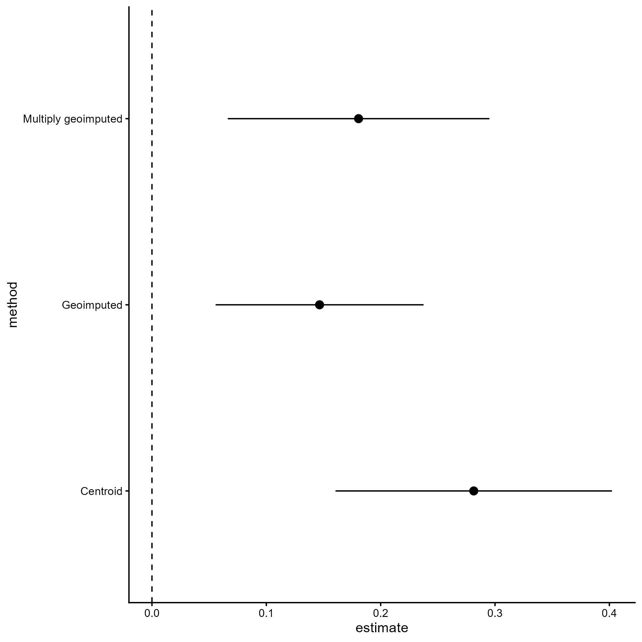
The coefficient plot shows the rent coefficient under each approach. The multiple geoimputation estimate accounts for both sampling uncertainty and location uncertainty. Its confidence interval is typically wider than the single imputation estimate but reflects what the data actually support. Consistent with Arbia’s law of geography, the aggregated estimate has a higher coefficient than the geoimputed and hence noisier approach. Additionally, the simple geoimputation seems to slightly underestimate the relationship.
res_comb <- bind_rows(
  `Centroid` = res_agg,
  `Geoimputed` = res_simple,
  `Multiply geoimputed` = res_mi,
  .id = "method"
) |>
  filter(term == "rent")

ggplot(res_comb) +
  geom_vline(xintercept = 0, linetype = "dashed") +
  geom_pointrange(aes(
    x = estimate,
    y = method,
    xmin = conf.low,
    xmax = conf.high
  )) +
  scale_y_discrete(breaks = c("Multiply geoimputed", "Geoimputed", "Centroid")) +
  theme_classic()