Administrative areas — bkg

Retrieve polygon geometries of administrative areas in Germany. All administrative levels are supported at different spatial resolutions.

bkg_admin interfaces a WFS that allows prefiltering but provides no historical data and allows a maximum scale of 1:250,000.
bkg_admin_archive allows access to historical data but has no prefiltering.
bkg_admin_highres (vg25) allows access to high-resolution data going as low as 1:25,000 but allows no prefiltering.

These functions interface the vg* products of the BKG.

Usage

bkg_admin(
  ...,
  level = "krs",
  scale = c("250", "1000", "2500", "5000"),
  key_date = c("0101", "1231"),
  bbox = NULL,
  poly = NULL,
  predicate = "intersects",
  filter = NULL,
  epsg = 3035,
  properties = NULL,
  max = NULL
)

bkg_admin_archive(
  level = "krs",
  scale = c("250", "1000", "2500", "5000"),
  key_date = c("0101", "1231"),
  year = "latest",
  timeout = 120,
  update_cache = FALSE
)

bkg_admin_highres(
  level = "krs",
  year = "latest",
  layer = NULL,
  timeout = 600,
  update_cache = FALSE
)

Arguments

...

Used to construct CQL filters. Dot arguments accept an R-like syntax that is converted to CQL queries internally. These queries basically consist of a property name on the left, an aribtrary vector on the right, and an operator that links both sides. If multiple queries are provided, they will be chained with AND. The following operators and their respective equivalents in CQL and XML are supported:

R	CQL	XML
`==`	`=`	`PropertyIsEqualTo`
`!=`	`<>`	`PropertyIsNotEqualTo`
`<`	`<`	`PropertyIsLessThan`
`>`	`>`	`PropertyIsGreaterThan`
`>=`	`>=`	`PropertyIsGreaterThanOrEqualTo`
`<=`	`<=`	`PropertyIsLessThanOrEqualTo`
`%LIKE%`	`LIKE`	`PropertyIsLike`
`%ILIKE%`	`ILIKE`
	`%in%`	`IN`

To construct more complex queries, you can use the filter argument to pass CQL queries directly. Also note that you can switch between CQL and XML queries using options(ffm_query_language = "xml"). See also wfs_filter.

level

Administrative level to download. Must be one of "sta" (Germany), "lan" (federal states), "rbz" (governmental districts), "krs" (districts), "vwg" (administrative associations), "gem" (municipalities), "li" (boundary lines), or "pk" (municipality centroids). Defaults to districts.

scale

Scale of the geometries. Can be "250" (1:250,000), "1000" (1:1,000,000), "2500" (1:2,500,000) or "5000" (1:5,000,000). If "250", population data is included in the output. Defaults to "250".

key_date

For resolution %in% c("250", "5000"), specifies the key date from which to download administrative data. Can be either "0101" (January 1) or "1231" (December 31). The latter is able to georeference statistical data while the first integrates changes made in the new year. If "1231", population data is attached, otherwise not. Note that population data is not available at all scales (usually 250 and 1000). Defaults to "0101".

bbox

An sf geometry or a boundary box vector of the format c(xmin, ymin, xmax, ymax). Used as a geometric filter to include only those geometries that relate to bbox according to the predicate specified in predicate. If an sf geometry is provided, coordinates are automatically transformed to ESPG:25832 (the default CRS), otherwise they are expected to be in EPSG:25832.

poly

An sf geometry. Used as a geometric filter to include only those geometries that relate to poly according to the predicate specified in predicate. Coordinates are automatically transformed to ESPG:25832 (the default CRS).

predicate

A spatial predicate that is used to relate the output geometries with the object specified in bbox or poly. For example, if predicate = "within", and bbox is specified, returns only those geometries that lie within bbox. Can be one of "equals", "disjoint", "intersects", "touches", "crosses", "within", "contains", "overlaps", "relate", "dwithin", or "beyond". Defaults to "intersects".

filter

A character string containing a valid CQL or XML filter. This string is appended to the query constructed through .... Use this argument to construct more complex filters. Defaults to NULL.

epsg

An EPSG code specifying a coordinate reference system of the output. If you're unsure what this means, try running sf::st_crs(...)$epsg on a spatial object that you are working with. Defaults to 3035.

properties

Vector of columns to include in the output.

max

Maximum number of results to return.

year

Version year of the dataset. You can use latest to retrieve the latest dataset version available on the BKG's geodata center. Older versions can be browsed using the archive.

timeout

Timeout value for the data download passed to req_timeout. Adjust this if your internet connection is slow or you are downloading larger datasets.

update_cache

By default, downloaded files are cached in the tempdir() directory of R. When downloading the same data again, the data is not downloaded but instead taken from the cache. Sometimes this can be not the desired behavior. If you want to overwrite the cache, pass TRUE. Defaults to FALSE, i.e. always adopt the cache if possible.

layer

The vg25 product used in bkg_admin_highres contains a couple of metadata files. You can set a layer name to read these files, otherwise the main file is read.

Value

An sf dataframe with multipolygon geometries and different columns depending on the geometry type. Areal geometries generally have the following columns:

objid: Unique object identifier
beginn: Creation of the object in the DLM
ade: Integer representing the administrative level. Can be one of
- 1: Germany
- 2: Federal state
- 3: Governmental district
- 4: District
- 5: Administrative association
- 6: Municipality
gf: Integer representing the geofactor; whether an area is "structured" or not. Land is structured if it is part of a state or other administrative unit but is not further divided into administrative units. Can be one of
- 1: Unstructured, waterbody
- 2: Structured, waterbody
- 3: Unstructured, land
- 4: Structured, land
bsg: Special areas, can be 1 (Germany) or 9 (Lake Constance)
ars: Territorial code (Amtlicher Regionalschlu00fcssel). The ARS is stuctured hierarchically as follows:
- Position 1-2: Federal state
- Position 3: Government region
- Position 4-5: District
- Position 6-9: Administrative association
- Position 10-12: Municipality
ags: Official municipality key (Amtlicher Gemeindeschlu00fcssel). Related to the ARS but shortened to omit position 6 to 9. Structured as follows:
- Position 1-2: Federal state
- Position 3: Government region
- Position 4-5: District
- Position 6-8: Municipality
sdv_ars: ARS of the seat of administration
gen: Geographical name
bez: Label of the administrative unit
ibz: Identifier of the label
bem: Comment on the label
nbd: Formation of the geographical name. Can be "ja" if the label is part of the name or "nein" otherwise.
nuts: NUTS identifier based on the Eurostat regional classification
ars_0: ARS identifier with trailing zeroes
ags_0: AGS identifier with trailing zeroes
wsk: Legally relevant date for the effectiveness of administrative changes
sn_l: Country component of the ARS
sn_r: Governmental district component of the ARS
sn_k: District component of the ARS
sn_v1: First part of the administrative association component of the ARS
sn_v2: Second part of the administrative association component of the ARS
sn_g: Municipality component of the ARS
fk_3: Purpose of the third key position. If "R", indicates the government region, if "K", indicates the district
dkm_id: Identifier in the digital landscape model (DLM250)
ewz: Number of inhabitants
kfl: Land register area in square kilometers

Boundary geometries ("li" can have additional columns:

agz: Type of border. Can be one of
- 1: National border
- 2: State border
- 3: Governmental district border
- 4: District border
- 5: Administrative association border
- 6: Municipality border
- 9: Coastline
rdg: Legal definition of a border. Can be 1 (determined), 2 (not determined) or 9 (coastline)
gm5: Border characteristic of administrative association borders (AGZ 5). Used to describe the purpose of these borders. Can be 0 (characteristics by AGZ) or 8 (non-association border)
gmk: Border characteristic by coast/ocean. Specifies whether a border runs a long a waterbody. Can be one of
- 7: borders on the ocean
- 8: auxiliary borders on the ocean
- 9: borders at the coastline
- 0: no characteristics
dlm_id: Identifier in the digital landscape model (DLM250)

Point geometries ("pk") have the following additional columns:

otl: Name of the locality in the digital landscale model (DLM250)
lon_dez: Decimal longitude
lat_dez: Decimal latitude
lon_gms: Geographical longitude
lat_gms: Geographical latitude

Query language

By default, WFS requests use CQL (Contextual Query Language) queries for simplicity. CQL queries only work together with GET requests. This means that when the URL is longer than 2048 characters, they fail. While POST requests are much more flexible and able to accommodate long queries, XML is really a pain to work with and I'm not confident in my approach to construct XML queries. You can control whether to send GET or POST requests by setting options(ffm_query_language = "XML") or options(ffm_query_language = "CQL").

Examples

if (FALSE) { # getFromNamespace("ffm_run_examples", ns = "ffm")()
# You can use R-like operators to query the WFS
bkg_admin(ags %LIKE% "05%") # districts in NRW
bkg_admin(sn_l == "05") # does the same thing
bkg_admin(gen %LIKE% "Ber%") # districts starting with Ber*

# To query population and area, the key date must be December 31
bkg_admin(ewz > 500000, key_date = "1231") # districts over 500k people
bkg_admin(kfl <= 100, key_date = "1231") # districts with low land register area

# Using `gf == 9`, you can exclude waterbodies like oceans
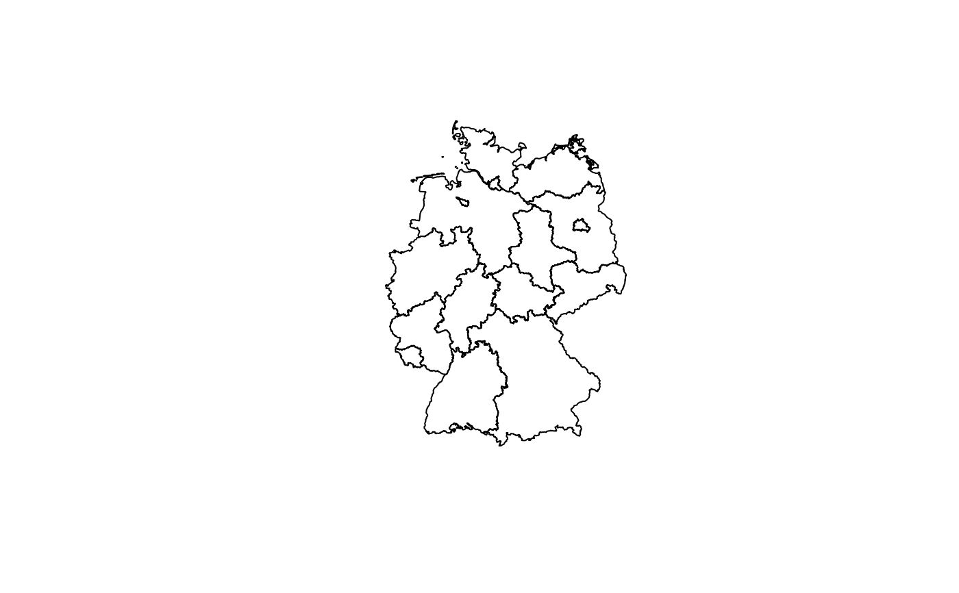
states <- bkg_admin(scale = "5000", level = "lan", gf == 9)
plot(states$geometry)

# Download historical data
bkg_admin_archive(scale = "5000", level = "sta", year = "2021")

if (FALSE) { # \dontrun{
# Download high-resolution data (takes a long time!)
bkg_admin_highres(level = "lan")
} # }
}